You can find the codes from this:
- Backpropagation and Overfitting
- Using Pytorch and CNN
- Fine-tuning a pretrained CNN
- CNN Visualization: Deep Features, Attention Maps
- Adversarial Patterns and Attacks
- Gaussian Variational Autoencoders
- Metric Learning for COVID-19
- Chatbot with Pretrained Models
- Train Your NLP Models by Transformer
- Using AI in Applications
C:\Users\hunter\Documents\MyGithub\hexo-chengkang\source\img\article\DeepLearningImages\Lab1
Backpropagation and Overfitting
You can find the code from github.

In the above figure, we set $w_{ij}^{(k)}$, and $k \in {(1,2)}$, $i \in {(1,2,3,4)}$, $j \in {(1,2,3,4})$. The actication functions in the input and the output layers are linear functions: $f_{(0)}(s)=s$, $f_{(2)}(s)=s$, and the actication functions in the hidden layers is a linear functions: $f_{(0)}(s)=0.1s$. Then, the input is $(x_{1}^{(0)},x_{2}^{(0)})=(1,1)$, the expected output is $(d_{1},d_{2},d_{3})=(1,2,3)$, and the learning rate $\mu$ is $0.1$.
The output of the neural network
The output of the hidden layer
$x_{1}^{(1)}=f_{(1)}(w_{11}^1x_{1}^{(0)}+w_{21}^1x_{2}^{(0)})=0.1 \times (1 \times 1+2 \times 1)=0.3$
$x_{2}^{(1)}=f_{(1)}(w_{12}^1x_{1}^{(0)}+w_{22}^1x_{2}^{(0)})=0.1 \times (1 \times 1+2 \times 1)=0.3$
$x_{3}^{(1)}=f_{(1)}(w_{13}^1x_{1}^{(0)}+w_{23}^1x_{2}^{(0)})=0.1 \times (1 \times 1+2 \times 1)=0.3$
$x_{4}^{(1)}=f_{(1)}(w_{14}^1x_{1}^{(0)}+w_{24}^1x_{2}^{(0)})=0.1 \times (1 \times 1+2 \times 1)=0.3$
The output of the output layer
$x_{1}^{(2)}=f_{(2)}(w_{11}^2x_{1}^{(1)}+w_{21}^2x_{2}^{(1)}+w_{31}^2x_{3}^{(1)}+w_{41}^2x_{4}^{(1)})=1 \times (1 \times 0.3 \times 4)=1.2$
$x_{2}^{(2)}=f_{(2)}(w_{12}^2x_{1}^{(1)}+w_{22}^2x_{2}^{(1)}+w_{32}^2x_{3}^{(1)}+w_{42}^2x_{4}^{(1)})=1 \times (2 \times 0.3 \times 4)=2.4$
$x_{3}^{(2)}=f_{(2)}(w_{13}^2x_{1}^{(1)}+w_{23}^2x_{2}^{(1)}+w_{33}^2x_{3}^{(1)}+w_{43}^2x_{4}^{(1)})=1 \times (1 \times 0.3 \times 4)=1.2$
The update of weights during the backpropagation
The error of the output layer
$\delta_{1}^{(2)}=(d_{1}-x_{1}^{(2)})f_{(2)}^{’}(s_{1}^{(2)})=(1-1.2) \times 1=-0.2$
$\delta_{2}^{(2)}=(d_{2}-x_{2}^{(2)})f_{(2)}^{’}(s_{2}^{(2)})=(2-2.4) \times 1=-0.4$
$\delta_{3}^{(2)}=(d_{3}-x_{3}^{(2)})f_{(2)}^{’}(s_{3}^{(2)})=(1-1.2) \times 1=-0.2$
The error of the hidden layer
$\delta_{1}^{(1)}=f_{(1)}^{’}(s_{1}^{(1)}) \sum_{k=1}^{3} \delta_{k}^{(2)} w_{1k}^{(2)}=0.1 \times (-0.2 \times 1-0.4 \times 2-0.2 \times 1)=-0.12$
$\delta_{2}^{(1)}=f_{(1)}^{’}(s_{2}^{(1)}) \sum_{k=1}^{3} \delta_{k}^{(2)} w_{2k}^{(2)}=0.1 \times (-0.2 \times 1-0.4 \times 2-0.2 \times 1)=-0.12$
$\delta_{3}^{(1)}=f_{(1)}^{’}(s_{3}^{(1)}) \sum_{k=1}^{3} \delta_{k}^{(2)} w_{3k}^{(2)}=0.1 \times (-0.2 \times 1-0.4 \times 2-0.2 \times 1)=-0.12$
$\delta_{4}^{(1)}=f_{(1)}^{’}(s_{4}^{(1)}) \sum_{k=1}^{3} \delta_{k}^{(2)} w_{4k}^{(2)}=0.1 \times (-0.2 \times 1-0.4 \times 2-0.2 \times 1)=-0.12$
The weight update between the output layer and the hidden layer
$w_{11}^{(2)}[1]=w_{11}^{(2)}[0]+ \mu \delta_{1}^{(2)}x_{1}^{(1)}=1+0.1 \times (-0.2) \times 0.3=0.994$
then $w_{21}^{(2)}[1]=w_{31}^{(2)}[1]=w_{41}^{(2)}[1]=0.994$.
$w_{12}^{(2)}[1]=w_{12}^{(2)}[0]+ \mu \delta_{2}^{(2)}x_{1}^{(1)}=2+0.1 \times (-0.4) \times 0.3=1.988$
then $w_{22}^{(2)}[1]=w_{32}^{(2)}[1]=w_{42}^{(2)}[1]=1.988$.
$w_{13}^{(2)}[1]=w_{13}^{(2)}[0]+ \mu \delta_{3}^{(2)}x_{1}^{(1)}=1+0.1 \times (-0.2) \times 0.3=0.994$
then $w_{23}^{(2)}[1]=w_{33}^{(2)}[1]=w_{43}^{(2)}[1]=0.994$.
The weight update between the input layer and the hidden layer
$w_{11}^{1}[1]=w_{11}^{1}[0]+ \mu \delta_{1}^{(1)}x_{1}^{(0)}=1+0.1 \times (-0.12) \times 1=0.988$
$w_{12}^{1}[1]=w_{12}^{1}[0]+ \mu \delta_{2}^{(1)}x_{1}^{(0)}=1+0.1 \times (-0.12) \times 1=0.988$
$w_{13}^{1}[1]=w_{13}^{1}[0]+ \mu \delta_{3}^{(1)}x_{1}^{(0)}=1+0.1 \times (-0.12) \times 1=0.988$
$w_{14}^{1}[1]=w_{14}^{1}[0]+ \mu \delta_{4}^{(1)}x_{1}^{(0)}=1+0.1 \times (-0.12) \times 1=0.988$
$w_{21}^{1}[1]=w_{21}^{1}[0]+ \mu \delta_{1}^{(1)}x_{2}^{(0)}=2+0.1 \times (-0.12) \times 1=1.988$
$w_{22}^{1}[1]=w_{22}^{1}[0]+ \mu \delta_{2}^{(1)}x_{2}^{(0)}=2+0.1 \times (-0.12) \times 1=1.988$
$w_{23}^{1}[1]=w_{23}^{1}[0]+ \mu \delta_{3}^{(1)}x_{2}^{(0)}=2+0.1 \times (-0.12) \times 1=1.988$
$w_{24}^{1}[1]=w_{24}^{1}[0]+ \mu \delta_{4}^{(1)}x_{2}^{(0)}=2+0.1 \times (-0.12) \times 1=1.988$
Those above steps are the first round weights updating, and then continue the second, the third…until they satisfy the constrain requirement.
Using Pytorch and CNN
You can find the code from github.
Getting Started
What is PyTorch: python front end, C++ libraries (A10), Target devices libraries (cuDNN). These will be useful resources for this task:
- Installing PyTorch. Develop and debug locally with CPU/GPU on any system. Choose a CUDA version, important to be able to write generic code.
- PyTorch docs.
Use this script mnist.py, and the history.pickle, the dictionary checkpoint_epoch1.checkpoint, model_cuda.pth, and the optimizer_cuda.pth are saved in the result fold.
Train and Test
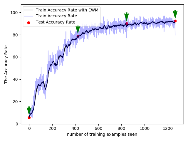
You can use this script plot_loss_train_curve.py to draw loss and train curves. This figure below shows the accuracy curve and the loss curve. Red dot are the accuracy (loss in the right panel) curve using Test dataset after each one epoch. Black line is the accuracy curve (loss in the right panel) with exponentially weighted average (EWA), and the partially transparant blue line is the raw accuracy (loss in the right panel) curve.
| Accuracy Curve | Loss Curve |
|---|---|
 |
 |
tSNE, Confusion Matrix and ROC Curve
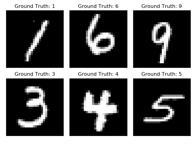
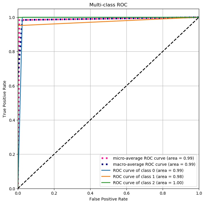
You can use this script plot_tSNE.py to tSNE, Confusion Matrix and ROC Curve. For the rSNE, although the boundary is not so perfect, after using nearest neighbor classifier, the accuracy rate can reach 0ver 90%.
| Example | tSNE |
|---|---|
 |
 |
Confusion Matrix

ROC Curve

Fine-tuning a Pretrained CNN
You can find the code from github.
You can use one of the following models: VGG11 and Squeezenet.
Download one of the example datasets for this task:
-
Butterflies (35Mb)
-
iNaturalist mix1 (108Mb)
All of the datasets contain color images 224×224 pixels of 10 categories.
For example, different learning rates can effect the accuracy and loss curves .
| Leaerning Rate | Accuracy Curve |
|---|---|
| lr=0.0001 |  |
| lr=0.01 |  |
| lr=1 |  |
CNN Visualization: Deep Features, Attention Maps
You can find the code from github.
For this task we need just one image from ImageNet. We provide an image of a labrador retriever.

Besides we need the class codes for the 1000 categories in ImageNet. We provide it as text file imagenet_classes.txt
Visualise the input image and the transformed
Load the image, apply the classifier and report the top 10 classes. Visualise the input image and the transformed (resampled & normalised) tensor image. For the latter you may use the make_grid function mentioned above.
Feature maps.

Gradien maps.

Activations of a given layer (activation_max_layer6]).

Adversarial Patterns and Attacks
You can find the code from github.
In this task, you should choose a clean image which is correctly classified by the net (e.g. the image of the labrador retriever). And then, choose a target class different from the true class (e.g. 892: wall clock) and fix an ε > 0. Implement a projected gradient ascent that aims to maximize the softmax output of the target class w.r.t. the input image, but constrains the search to the ε-ball around the clean image. You can find a text file about the category list: imagenet_classes.txt.
The sample is labrador retriever.

Fast Gradient Sign Method
Let’s say we have an input X, which is correctly classified by our model ($M$). We want to find an adversarial example $\widehat{X}$, which is perceptually indistinguishable from original input X, such that it will be misclassified by that same model ($M$). We can do that by adding an adversarial perturbation ($\theta$) to the original input. Note that we want adversarial example to be indistinguishable from the original one. That can be achieved by constraining the magnitude of adversarial perturbation: $|X-\widehat{X} |_{\infty} \leqslant \epsilon$.
That is, the $L_{\infty}$ norm should be less than epsilon. Here, $L_{\infty}$ denotes the maximum changes for all pixels in adversarial example. Fast Gradient Sign Method (FGSM) is a fast and computationally efficient method to generate adversarial examples. However, it usually has a lower success rate. The formula to find adversarial example is as follows:
$X^{adv}=X+\epsilon \cdot sign(\nabla_{X}J(X,Y_{true}))$
Here,
$X$ = original (clean) input
$X^{adv}$ = adversarial input (intentionally designed to be misclassified by our model)
$ϵ$ = magnitude of adversarial perturbation
$\nabla_{X}J(X,Y_{true})$ = gradient of loss function w.r.t to input ($X$)
The targeted result is:

Gaussian Variational Autoencoders
You can find the code from github.
The sample is the MNIST.

| Input with Noise | Output with Noise |
|---|---|
 |
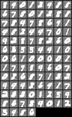 |
Metric Learning for COVID-19
You can find the code from github.
For an anchor (query) image $a$ let the positive example $p$ be of the same class and a negative example $n$ be of different class than $a$. We want that each positive example to be closer to the anchor than all negative examples (a margin $\alpha \geq 0$). The constraint is violated if $d(f_a,f_p)-d(f_a,f_n)+\alpha \geq 0$.
Accordingly we define the triplet loss as the total violation of these constraints:
$l_a=\sum_{p,n}max(d(f_a,f_p)-d(f_a,f_n)+\alpha)$
There you can find many loss functions for metric learning.
| Example | tSNE |
|---|---|
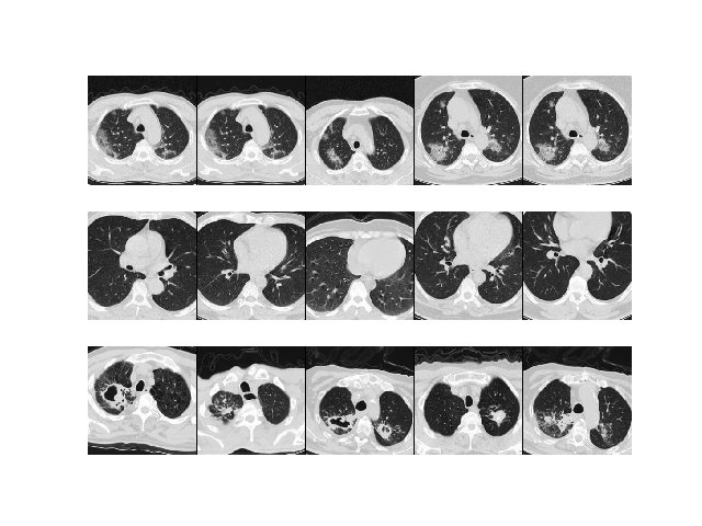 |
 |
| Confusion Matrix | ROC Curve |
|---|---|
 |
 |
Chatbot with Pretrained Models
You can find the code from github.
All of the necessary components to run this project are on the GitHub repository. Feel free to fork the repository and clone it to your local machine. Here’s a quick breakdown of the components:
- train_chatbot.py — the code for reading in the natural language data into a training set and using a Keras sequential neural network to create a model
- gui_chatbot.py — the code for cleaning up the responses based on the predictions from the model and creating a graphical interface for interacting with the chatbot
- classes.pkl — a list of different types of classes of responses
- words.pkl — a list of different words that could be used for pattern recognition
- intents.json — abunch of JavaScript objects that lists different tags that correspond to different types of word patterns
- chatbot_model.h5 — the actual model created by train_chatbot.py and used by gui_chatbot.py.
NOTICE: there, if you find that your NLTK cannot import the word_tokenize, and you found that all the packages are installed correctly, See link. And add the command nltk.download(‘punkt’) to your script.
Train Your NLP Models by Transformer
You can find the code from github.
Here is the original paper link about T5 https://arxiv.org/abs/1910.10683. And
T5 fine-tuning
This notebook is to showcase how to fine-tune T5 model with Huggigface’s Transformers to solve different NLP tasks using text-2-text approach proposed in the T5 paper. For demo I chose 3 non text-2-text problems just to reiterate the fact from the paper that how widely applicable this text-2-text framework is and how it can be used for different tasks without changing the model at all.
Setting Developing environment
The virtual developing python environment (python 3.6 + Pycharm).
Firstly, installing the virtual tool:
pip3 install virtualenv
And then,
virtualenv TestEnv
or
virtualenv --system-site-packages TestEnv
After that, you should activate the environment.
for Windows
source ./TestEnv /Script/activate
for Linux
source ./TestEnv /bin/activate
or quit the virtual environment
deactivate
Preprocessing
First, install the required packages:
pip install transformers
pip install pytorch_lightning
mkdir /workspace/working/t5_tweet
mkdir /workspace/input/tweetextract
We provide the dataset in:
/workspace/input/tweetextract/val.csv
/workspace/input/tweetextract/test.csv
/workspace/input/tweetextract/train.csv
Training and Chatting
You can find more detials about T5 mpdel from: https://huggingface.co/transformers/model_doc/t5.html
If you finished the preparatory work, you can excute the training by runing
python test_t5_gpu.py
or, if you only have cpus
python test_t5_cpu.py
After trainng several epoches, you can save the model in /workspace/woring/t5_tweet/. And call the model when using the chatbot by excuting:
python chatbot_gui.py
The Chatbot GUI:

Using AI in Applications
Please read this blog, and you will find a very interesting game.
Making an Interactive Running Game with Head or Body Movement Using TensorFlow.js
You can find the code from github.
| Contributor | |
|---|---|
| Cheng Kang | kangchen@fel.cvut.cz |
| Xujing Yao | xy147@leicester.ac.uk |